Examples

A 1D signal

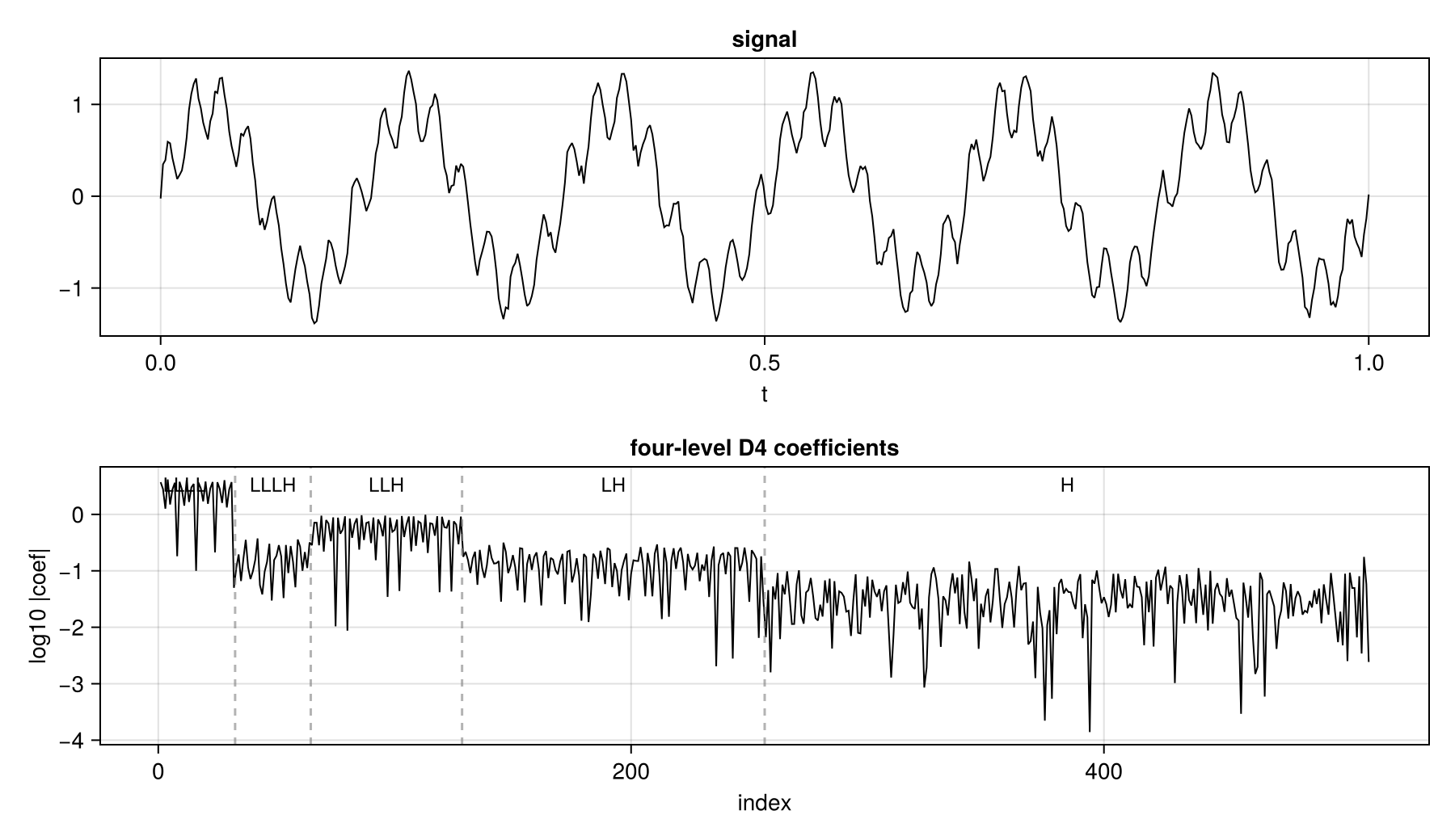
A four-level D4 transform splits a signal into one approximation band and four detail bands.

using NDWaveletTransforms
using Random

Random.seed!(1)
t = range(0, 1, length = 2048)
s = sin.(2pi .* 6 .* t) .+ 0.35 .* sin.(2pi .* 45 .* t) .+ 0.05 .* randn(2048)

c = dwt(s, WT_D4, 4)

Bands are named by their path from the root of the tree ("L" for lowpass, "H" for highpass). The strip below reads LLLL, LLLH, LLH, LH, H from coarsest to finest scales.

A signal and its DWT.

An image

img = rand(512, 512)
c = dwt(img, WT_D4, 3)

mags = sort(abs.(c); rev = true)
k = round(Int, 0.05 * length(c))
compressed = copy(c)
compressed[abs.(compressed) .< mags[k]] .= 0
img_compressed = idwt(compressed, WT_D4, 3)

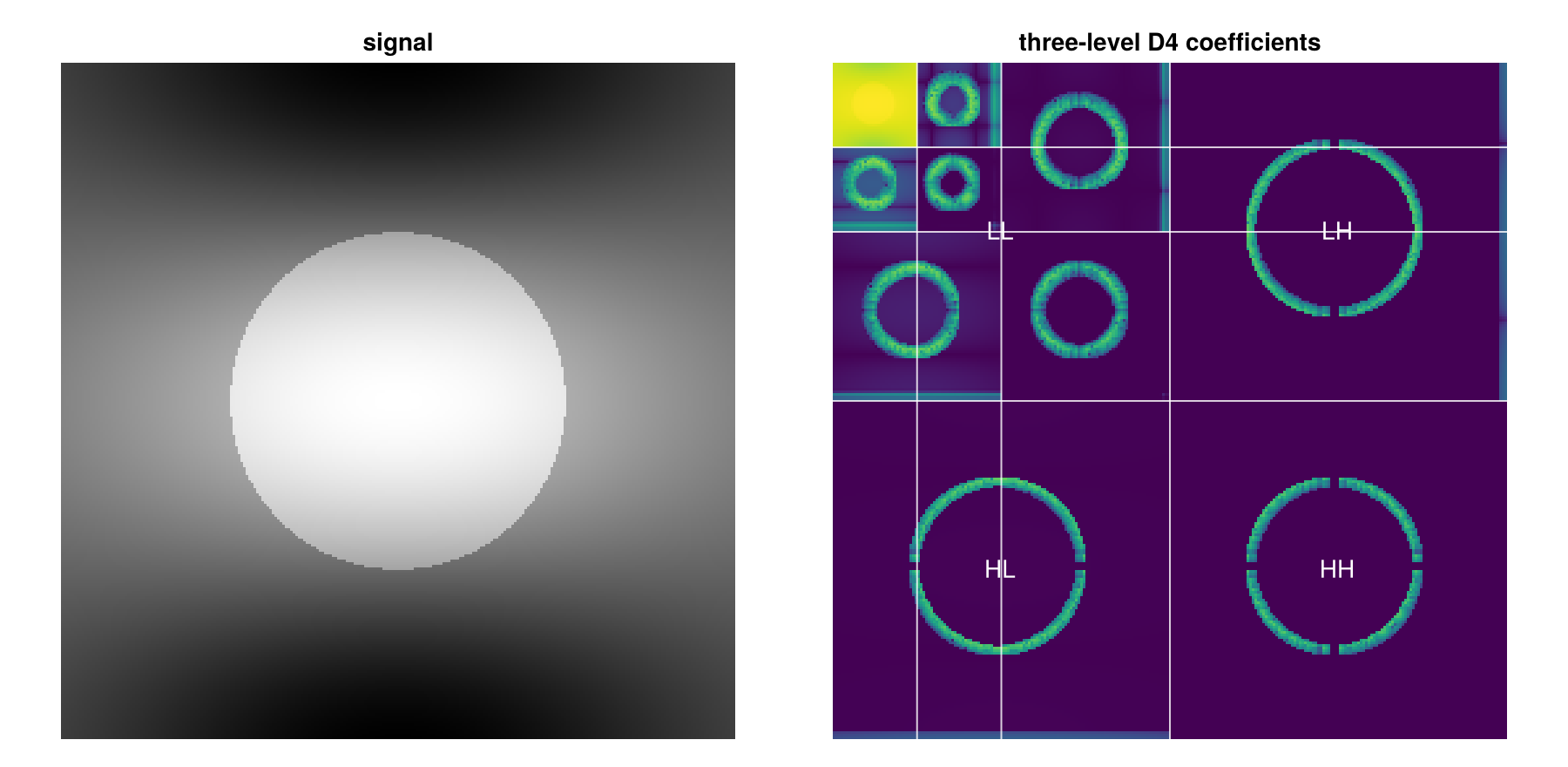
The coefficient array is an r-tree (a quadtree for a 2D transform, an octree for a 3D transform, etc.). In a conventional DWT, a multilevel transform recurses into the approximation band, shown in the top-left corner.

The subband tiling of a three-level transform.

Sparsity

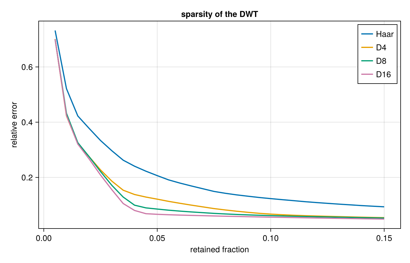
Smooth signals concentrate their energy in a few wavelet coefficients. Keeping the largest coefficients and zeroing the rest reconstructs the signal to a relative error that falls with the fraction kept. Filters with more vanishing moments do better on smooth signals, but have more taps, so are more sensitive to phase shfits.

$Relative error against the fraction of retained coefficients.$

Levels along each axis

The level argument can be a tuple, so a rectangular array can be transformed more deeply along one dimension than another.

img = rand(256, 256)
dwt(img, WT_D4, (1, 3))    # one level along axis 1, three along axis 2
dwt(img, WT_D4, (3, 1))    # the other way round

@rtview accept _ as a "do-nothing" index. This is helpful when operating on signals transformed to different levels in different dimensions: for instance, dwt!(x, WT_HAAR, (1,2)) might be indexed as @rtview x[:ll, :_h].

For instance, the following returns the approximation band of a (1,3) transform.

c = dwt(img, WT_D4, (1, 3))
@rtview c[:ll, :_l, :_l]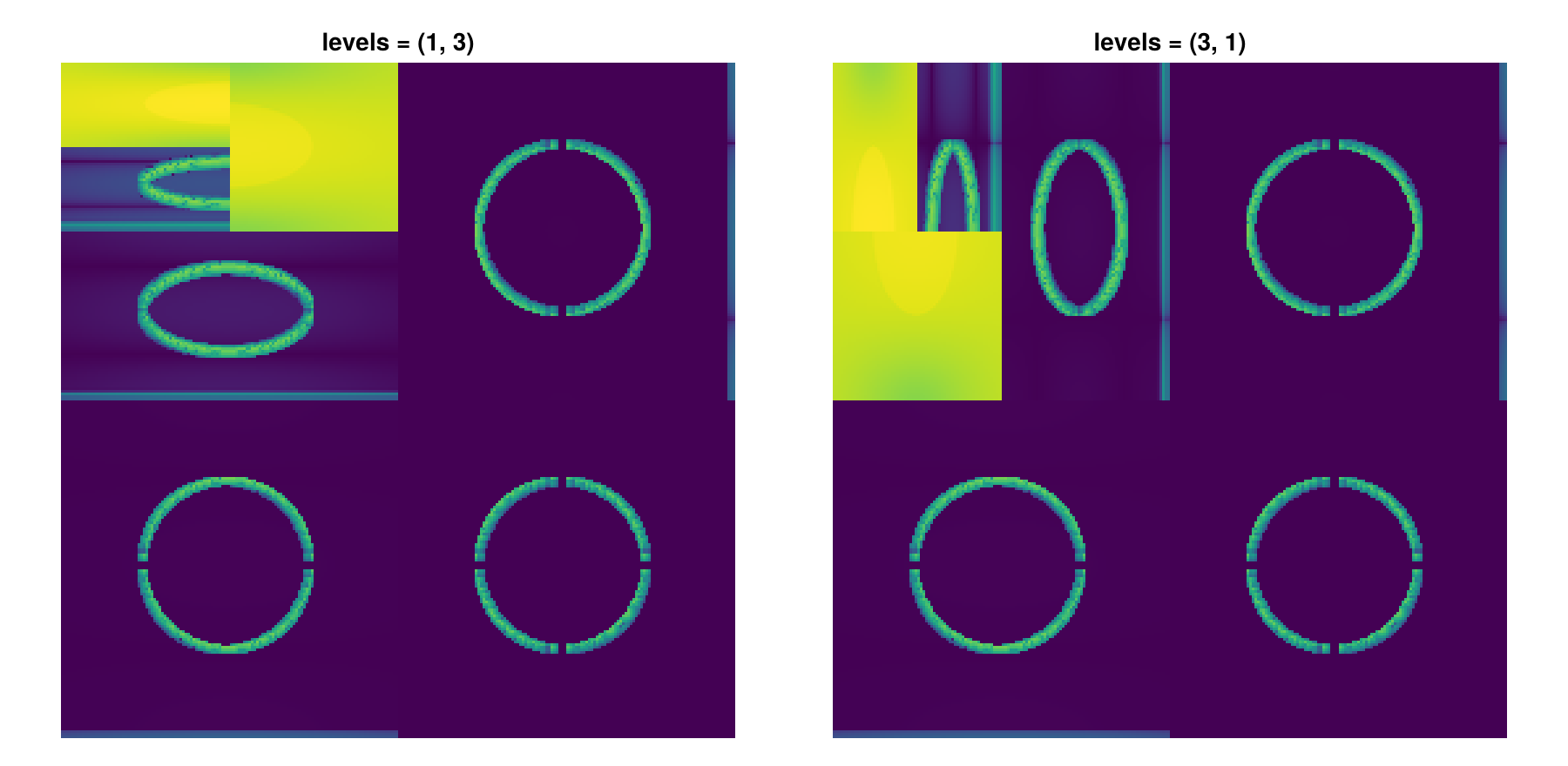

The same image at levels (1, 3) and (3, 1).

Transform flavours

Standard and nonstandard DWTs and WPTs are supported:

img = rand(128, 128)
dwt(img, WT_D4, 2)     # standard
wpt(img, WT_D4, 2)     # every subband recurses
nsdwt(img, WT_D4, 2)   # nonstandard ordering
nswpt(img, WT_D4, 2)   # both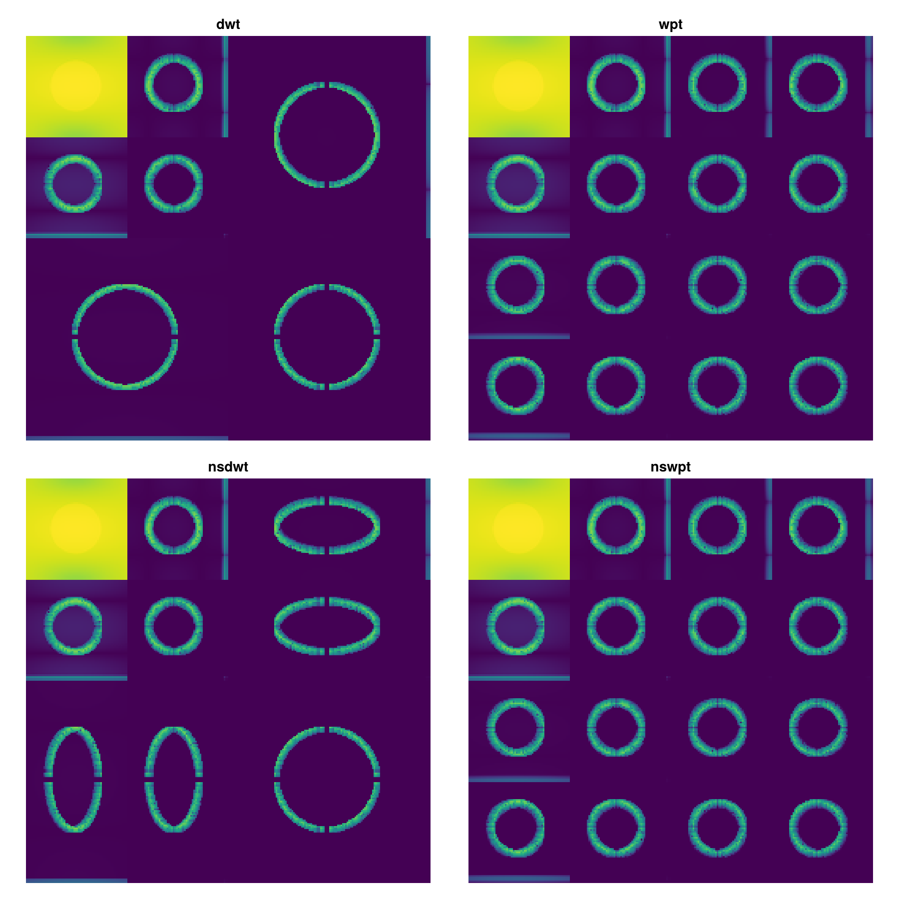

Four transform flavours.

The packet transform subdivides every subband, so the array is a full quad-tree rather than a corner of repeated approximation. The nonstandard ordering leaves a different arrangement in the detail bands.

A WPT inverts with iwpt and a nonstandard one with nsidwt, e.g.

x = rand(256)
c = wpt(x, WT_D4, 3)
iwpt!(c, WT_D4, 3)
c ≈ x